A Honeycomb Story: Five Different Kinds of Bar Charts
This blog entry continues my discussion of Designing With Data. You might enjoy Part I: “Designing With Data.”
I worked for Honeycomb.io as the first Design Researcher; I was brought in to help the company think about how data visualization could support data analytics.
At Honeycomb, I helped create an analysis tool called BubbleUp — there’s a great little video about it here. BubbleUp helps tame high-cardinality and high-dimensionality data by letting a user easily do hundreds of comparisons at a glance. With BubbleUp, its easy to see why some data is acting differently, because the different dimensions really pop out visually.
Today, I want to talk about three behind-the-scenes pieces of the BubbleUp project.
The Core Analysis Loop
When I arrived at Honeycomb, the company was struggling to explain to customers why they should take advantage of high cardinality, high dimensionality data – that is, events with many columns and many possible values. Honeycomb’s support for this data is a key differentiator. Unfortunately, it is hard to make an interface that makes it easy to handle that kind of data – users can feel they’re searching for a needle in a haystack, and often have trouble figuring out what questions will give them useful results.
Indeed, we saw users doing precisely that fishing: they would use the GROUP BY picker on dimension after dimension.
I interviewed several different users to understand this behavior. At heart, the question they were asking was, “Why was this happening?” and found that they were all struggling with the same core analysis loop : they had the implicit hypothesis that something was different between bad events and good events, but weren’t sure what it was.

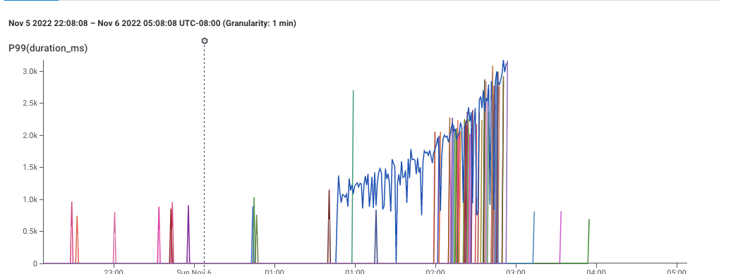
A graph showing 99th percentile latency for requests to a web service. Note that latency gradually increases to 2 seconds, then drops dramatically. This and following screenshots from Honeycomb.io
This, for example, is a screenshot of Honeycomb’s interface, showing the P99 of latency — that is, the speed of the slowest 1% of requests to a service. This gives a sense for how well the service is performing.
It’s pretty clear that something changed around 1:00 — the service started getting slower. This chart is an aggregation of individual events, each of which represents a request to the service. Each event in the dataset has lots of dimensions associated with it — the IP request of the requester, the operating system of the service, the name of the endpoint requested, and dozens of others — so its reasonable to believe that there is some dimension that is different.
It’s also pretty clear that the user can easily describe what happened: “some of the data is slower.” The user could point to the slow data and say “these ones! I want to know whether the events with latency over 1 second are different from the ones with latency around one second.”
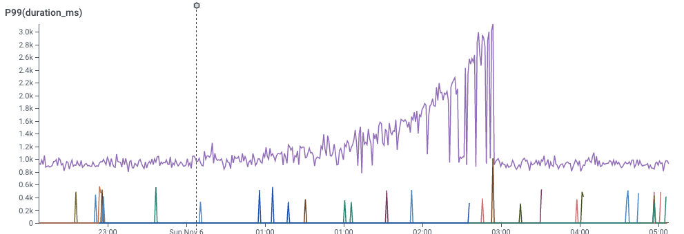
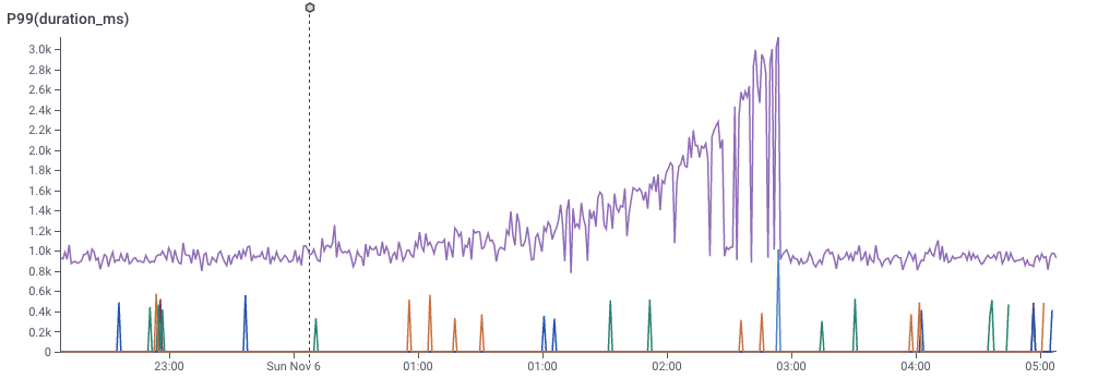
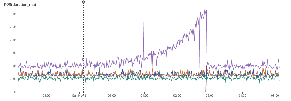
We can look at a different dimension by dividing the data with a GROUP BY.
In the slider below, I’ve picked a few of the dimensions and did a GROUP BY on them. You can see that some dimensions don’t really give good signal, but one of them really does. That dimension would be the key to the puzzle — What would it take to find that more easily?
(By the way — you can try this yourself, at Honeycomb’s sandbox, which comes pre-loaded with data to explore.)
Rapid Prototyping
I love histograms as an overview technique – they show all the different possible values of a dimension. They give a quick overview of what the data looks like, and they are easy to compare to each other. Better yet, for my purposes, they don’t take up much space.

These histograms do, fact, take up space on your bed when you cuddle with them. (Technically, these are “evil distributions,” visualzed as smooth histograms. These are from Nausisca Distributions, but unfortunately not for sale anymore.)
You can compare histograms in a couple of different ways: you can put them side-by-side, or you can overlay them. (The pillows illustrate overlaid histograms, with dotted lines showing different parameterized versions of the distributions.)
I pulled sample data from our dogfood system. The quickest tool I had at hand was to throw it into Google Sheets, and drew histograms one at a time, choosing whatever settings seemed to make something useful, and cutting and pasting them over each other. (I could tweak parameters later. Right now, it was time to just build out a version and see if it worked.) Even with this primitive approach, I could see that some dimensions were visibly different, which meant that maybe we could use this technique to explain why anomalies were happening.

One of the first sketches of comparing distributions in Google Sheets, comparing anomalous (orange) data to baseline (blue) data.
First, it’s pretty clear that there’s some signal here. The “endpoint” dimension shows that all of the orange data has the same endpoint! We’ve instantly located where the problem lies. Similarly, the “mysql_dur” dimension shows that the data of interest is much slower..
We can also see that there are a few tricks that will need to be resolved for this technique to work:
On the top-right, we see that the orange dataset has much less data than the blue dataset – perhaps only six values on that dimension. We’d definitely have to solve problems of making sure that the scales compared.
The middle-left shows a bigger problem: there’s only one distinct value for orange. It’s squinched up against the left side, which meant that I drew the orange in this sketch as a glow.
The fact that we got real data into even this low-fidelity sketch meant that we could start seeing whether our technique could work.
To learn more about future blockers, I implemented a second version as a Python notebook. That let me mass-produce the visualizations, and forced me to face the realities of the data. Axes turned into a mess. Lots of dimensions turned out to be really boring. Some dimensions had far too many distinct values to care about. Some had too few — or none at all.

An image from a python notebook prototyping BubbleUp.
The Python notebook let me start exploring in earnest. I added a handful of heuristics to the notebook to make them less terrible — hiding axes when there were too many values, dropping insignificant data, and scaling axes to match — and now we had something we could start experimenting with.
My first step was to build a manual testing process. I’d export data from a customer account, import it into the notebook, export the output as a PDF, and email the PDF to a customer. Laborious as it was, it got us feedback quickly.
This experience proved to me that it was our users were, in fact, able to identify anomalous behavior in their data — and that this visualization could pin it down.
Of course, that also meant we found yet more strange ways that our customer’s data behaved.
Handling Edge Cases
The version of BubbleUp Honeycomb ships today is very different from this primitive Python notebook. The early iterations helped us figure out where the challenges were going to be.
We came up with answers for …
Times when the two groups were radically different in size
Times when one group was sparsely populated, and the other was dense
How we order the bars, including which graphs should be alphabetical, numerical, or by value.
What we do about null values.
How we order the charts relative to each other.
One interesting implication is that BubbleUp today actually has five distinct code paths for drawing its histograms! (I certainly didn’t anticipate that when I put together that Google sheet.)
Low-cardinality string data is ordered by descending frequency of the baseline data, and gets an X axis
If there are more than 40 strings, we stop drawing the X axis
… and if there are more than ~75, we trim off the least common values, so the graph can show the most common of both the baseline and the outliers
Low-cardinality numeric data is not drawn proportionately, but is ordered by number — with HTTP error codes, for example, there’s no reason to have a big gap between 304 and 404.
High-cardinality, quantitative data is drawn as a continuous histogram, with overlapping (instead of distinct)) bars.
None of this would have been possible without getting data into the visualization rapidly, and iterating repeatedly: there’s simply no alternative to experimenting with user data, interviewing users, and iterating more.

The BubbleUp interface today. It’s gotten a lot better then that first Python notebook, and shows data in a much easier-to-understand way.